1. Python#
Python is a high-level programming language that allows you to express very powerful ideas in very few, readable, lines of code. It is one of the top three most used programming languages, competing with classical languages such as Java, C and C++. Besides being a great general-purpose programming language, thanks to a few popular libraries (e.g., pandas, numpy, scipy, matplotlib) Python has become a powerful environment for scientific computing.
1.1. Python versions and installation#
You will currently find two different versions of Python available, 2.7 and 3.x (where x is currently 9 or higher). This is due to the fact that Python 3.0 introduced many changes to the language that are incompatible with previous versions. That is, code written for Python 2.7 may not work under Python 3.x (and the other way around). For this reason, both versions are currently around. For this course we will use Python 3.x. So, make sure you have Python 3.x installed if you want to run code on your machine. Here you find precise installation instructions for specific operating system. If you are using MacOS or a Linux distribution the chances are high that Python is already installed on your machine.
1.2. Integrated Development Environment (IDE)#
It is recommended that you use an IDE for writing your Python files. This will simplify many tasks such as building a virtual environment and installing packages. There are many IDEs available. We recomment PyCharm which comes with many useful features. Follow the installation instructions to install it on your machine. Then follow these instructions on how to create a project.
1.3. Variables#
Much like mathematical variables, Python variables hold some value.
x = 2
print(x*3) # This does not change the content of the variable. The result of x*3 is not stored anywhere.
print(x) # x has not changed
6
2
The equal sign makes an assignment. The content on the right-hand side is assigned to the variable on the left-hand side. It should not be confused with the = sign in mathematics. The following expression does not make sense mathematically, as \(x\) satisfies this equation. In Python, this is a perfectly valid assignemetn.
x = x + 1
print(x)
3
Here you see that Python forgets how a value has been assigned. That is, \(x\) and \(y\) remain independent.
y = 7
print(y)

x = y + 1
print(x)

x = 10
print(x,y)
7
8
10 7
Similar to most programming languages, Python provides a number of basic data types. The most frequently used are integers, floats, booleans, and strings. If you learnt another programming language before such as Matlab or Java, these data types behave in a very similar way. However, unlike other programming languages, in Python you do not need to specify the type (i.e., Python is not a ``typed’’ language).
1.3.1. Numbers#
Integers and reals (or better floating-point numbers) work intuitively. Here are a few example of operations with numerical types.
x = 5
y = 2.5
print(x,y)
5 2.5
Get the data type.
print(type(x))
print(type(y))
<class 'int'>
<class 'float'>
Basic arithmetic operations.
print(x + 1)
print(x - 1)
print(x * 2)
print(x / 2)
6
4
10
2.5
Powers.
print(x ** 2)
25
Unary operators are operations applied to one variable only. The following changes the value stored in \(x\) to \(x+1\)
x += 1
print(x)
6
The following changes the value stored in \(x\) to \(x\cdot 2\).
x *= 2
print(x)
12
1.3.2. Booleans#
Python makes available all of the usual operators for Boolean logic with convenient English words rather than symbols.
t = True
f = False
print(type(t))
<class 'bool'>
print(t and f)
print(t or f)
print(not t)
False
True
False
The operator == stands for “is equal to”. It checks whether the content of two variables is the same.
Similarly, the operator != stands for “is not equal to”. It checks whether the content of two variables is different.
print(t == True)
print(t != f)
print(f == True)
True
True
False
1.3.3. Strings#
Python has many useful methods for manipulating strings. Strings can be created using single quotes or double quotes.
n = 'Numerical'
a = "Analysis"
print(n)
print(type(a))
Numerical
<class 'str'>
Here is how to get the length of a string.
print(len(a))
8
This is how to concatenate strings.
na = n + ' ' + a
print(na)
Numerical Analysis
These are examples of formatting strings. Say that we have three strings to print one after another, followed by a year.
s1 = "Course"
s2 = "Numerical"
s3 = "Analysis"
year = 2025
na = '%s %s %s %d' % (s1, s2, s3, year)

print(na)
Course Numerical Analysis 2025
We can also format floating-point numbers so that we show the desired number of decimal digits.
p ='Probability of success to two decimal digits %.2f' % (98.12345)
print(p)
p ='Probability of success to four decimal digits %.4f' % (98.12345)
print(p)
Probability of success to two decimal digits 98.12
Probability of success to four decimal digits 98.1235
Another possibility is to use f-strings or formatted strings. They allow you printing the content of variables directly.
operation1 = "addition"
a = 3
b = 2
operation2 = "product"
print(f"The result of the {operation1} is {b+a}")
print(f"The result of the {operation2} is {b*2}")
The result of the addition is 5
The result of the product is 4
Capitalization and upper-case.
s = 'hello'
print(s.capitalize())
print(s.upper())
Hello
HELLO
Replace a substring with another string, remove leading and trailing whitespaces.
print(s.replace('l', '(ell)'))
print('  world '.strip())
he(ell)(ell)o
world
Counting occurrences of a letter.
print(f"Number of %s in NumIntro" % 'i')
print("NumIntro".count("i"))
print(f"Number of %s in NumIntro" % 'I')
print("NumIntro".count("I"))
Number of i in NumIntro
0
Number of I in NumIntro
1
Looping through strings.
for i in na:
    print(i)
C
o
u
r
s
e

N
u
m
e
r
i
c
a
l

A
n
a
l
y
s
i
s

2
0
2
5
1.4. Data containers#
Often we would like to store a collection of data rather than individual variables. Python offers several types of containers according to the specific need.
1.4.1. Lists#
Lists represent vectors of data. They are typically (but not necessarily) used to store homogeneous data.
l = [10, 21, 42]
print(l)
[10, 21, 42]
List elements are accessed by their position. The first element is in position 0 and negative indices count from the end of the list.
print(l[1],l[0])
print(l[-1])
print(l[-3])
21 10
42
10
Lists may contain elements of different types
l[2] = 'NA'
print(l)
[10, 21, 'NA']
Unlike in other programming languages, Python lists may be resized. We can append new elements (i.e., add to the end of the list) and pop elements, i.e., remove and return the last element of the list
l.append('numIntro')
print(l)
x = l.pop()
print(x)
print(l)
[10, 21, 'NA', 'numIntro']
numIntro
[10, 21, 'NA']
A range can be used to efficiently create lists (see more https://docs.python.org/3.7/library/stdtypes.html#ranges).
A range of \(n\) will consists of the integers from \(0\) to \(n-1\). We can also specify the first and last number and the increment.
numbers_from_0_to_9 = list(range(10))
print(numbers_from_0_to_9)
numbers_from_1_to_5 = list(range(1,6))
print(numbers_from_1_to_5)
numbers_from_1_to_10 = list(range(1,10,2))
print(numbers_from_1_to_10)
[0, 1, 2, 3, 4, 5, 6, 7, 8, 9]
[1, 2, 3, 4, 5]
[1, 3, 5, 7, 9]
You canslice lists i.e., extract a sublist.
nums = list(range(5))
print(nums)
# Get a slice from position 2 (inclusive) to 4 (exclusive)
print(nums[2:4])
# Get a slice from index 2 to the end
print(nums[2:])
# Get a slice from the start to index 2 (exclusive)
print(nums[:2])
# Get a slice of the whole list
print(nums[:])
# Slice indices can be negative (remember that negative indices count from the end of the list)
print(nums[:-1])
# Assign a new sublist to a slice
nums[2:4] = [8, 9]
print(nums)
[0, 1, 2, 3, 4]
[2, 3]
[2, 3, 4]
[0, 1]
[0, 1, 2, 3, 4]
[0, 1, 2, 3]
[0, 1, 8, 9, 4]
You can loop over lists
animals = ['cat', 'dog', 'monkey']
for animal in animals:
    print(animal)

# If you also want to access the index of the elements
for idx, animal in enumerate(animals):
    print('#%d: %s' % (idx, animal))
cat
dog
monkey
#0: cat
#1: dog
#2: monkey
You can check if a list contains an element using the keyword in
print('cat' in animals)
print('tiger' in animals)
print('dog' not in animals)
True
False
False
When programming, frequently we want to transform one type of data into another. List comprehension provides a shorthand for this kind of tasks. As a simple example, the following code provides two equivalent ways (without and with list comprehension) of computing the square of the numbers in an existing list:
nums = [0, 1, 2, 3, 4]
squaresA = []

# Without list comprehension
for x in nums:
    squaresA.append(x ** 2)
print(squaresA)

# With list comprehension
squaresB = [x ** 2 for x in nums]
print(squaresB)

# With conditions (only the square of even numbers)
even_squares = [x ** 2 for x in nums if x % 2 == 0]
print(even_squares)
[0, 1, 4, 9, 16]
[0, 1, 4, 9, 16]
[0, 4, 16]
Summing lists of numbers
sum(even_squares)
20
1.4.2. Dictionaries#
A dictionary stores key-value pairs. These are examples of how to use them.
You may create a new dictionary with some data.
d = {'A': 10, 'B': 20}
Dictionaries can be created in a few alternative ways
d1 = dict(one=1, two=2, three=3)
d2 = {'one': 1, 'two': 2, 'three': 3}
d3 = dict([('two', 2), ('one', 1), ('three', 3)])
d4 = dict({'three': 3, 'one': 1, 'two': 2})
print(d1 == d2 == d3 == d4)
True
We can also create an empty dictionary and fill it later
dictionary = {}
dictionary['one'] = 1
dictionary['two'] = 2
print(dictionary)
{'one': 1, 'two': 2}
Get an entry from a dictionary
print(dictionary['one'])
1
Check if a dictionary has a given key
print('cat' in d)
print('A' in d)
False
True
Set an entry in a dictionary
d['C'] = '40'
print(d['C'])
40
Remove an element from a dictionary
del d['A']
print(d)
{'B': 20, 'C': '40'}
We can access the keys as follows
b = {'one': 1, 'two': 2, 'three': 3}
b.keys()
dict_keys(['one', 'two', 'three'])
Or, if we want the keys as a list
list(b.keys())
['one', 'two', 'three']
Similarly for the values
b.values(), list(b.values())
(dict_values([1, 2, 3]), [1, 2, 3])
This can be used to check if a value or a key is in the dictionary
print(1 in b.values())
print('one' in b.keys())
print('four' in b.keys())
print("one" in b)
True
True
False
True
You can iterate over the keys in a dictionary:
d = {'person': 2, 'cat': 4, 'spider': 8}
for animal in d:
    legs = d[animal]
    print('A %s has %d legs' % (animal, legs))
A person has 2 legs
A cat has 4 legs
A spider has 8 legs
If you want access to keys and their corresponding values, use the items method:
d.items()
dict_items([('person', 2), ('cat', 4), ('spider', 8)])
d = {'person': 2, 'cat': 4, 'spider': 8}
for animal, legs in d.items():
    print('A %s has %d legs' % (animal, legs))
A person has 2 legs
A cat has 4 legs
A spider has 8 legs
Comprehensions allows you to easily construct dictionaries. The following code will create a dictionary that stores, for each number, its square, but only for the even numbers.
nums = [0, 1, 2, 3, 4]
even_num_to_square = {x: x ** 2 for x in nums if x % 2 == 0}
print(even_num_to_square)
{0: 0, 2: 4, 4: 16}
1.4.3. Sets#
A set is an unordered collection of distinct elements.
animals = {'cat', 'dog'}
print(animals)
{'cat', 'dog'}
Check if an element is in a set
print('cat' in animals)
print('fish' in animals)
True
False
Number of elements in a set
print(len(animals))
2
Add an element to a set (adding an element that is already in the set does nothing)
animals.add('fish')
print('fish' in animals)
animals.add('cat')
print(animals)
print(len(animals))
True
{'cat', 'dog', 'fish'}
3
Remove an element from a set
animals.remove('cat')
print(len(animals))
print(animals)
2
{'dog', 'fish'}
Iterating over a set has the same syntax as iterating over a list; however since sets are unordered, you cannot make assumptions about the order in which you visit the elements of the set:
animals = {'cat', 'dog', 'fish'}
for idx, animal in enumerate(animals):
    print('#%d: %s' % (idx + 1, animal))
#1: cat
#2: dog
#3: fish
Like lists and dictionaries, we can easily construct sets using set comprehensions. The following code creates the set of squares of the numbers from 0 to 9. That is, all the numbers from \(0^2\) to \(9^2\) are there, but unordered.
nums = {x*x for x in range(10)}
print(nums)
{0, 1, 64, 4, 36, 9, 16, 49, 81, 25}
1.4.4. Tuples#
A tuple is an ordered list of values. A tuple is in many ways similar to a list; one of the most important differences is that tuples can be used as keys in dictionaries and as elements of sets, while lists cannot. However, tuples are immutable: you can’t change which variables they contain after construction. Here is a trivial example:
t = (5, 6)
print(type(t))
print(t)
<class 'tuple'>
(5, 6)
Create a dictionary with tuple keys. The dict has keys \((x,x+1)\) and value \(x\), that is \(\{(0,1):1, (1,2):1, \ldots\}\)
d = {(x, x + 1): x for x in range(10)}
print(d)
print(d[t])
print(d[(1, 2)])
{(0, 1): 0, (1, 2): 1, (2, 3): 2, (3, 4): 3, (4, 5): 4, (5, 6): 5, (6, 7): 6, (7, 8): 7, (8, 9): 8, (9, 10): 9}
5
1
1.5. Functions#
Python functions are sequences of instructions that perform a given task. They are defined using the def keyword. For example:
def sign(x):
    if x > 0:
        return 'positive'
    elif x < 0:
        return 'negative'
    else:
        return 'zero'

for x in [-1, 0, 1]:
    print(sign(x))
negative
zero
positive
Functions can take optional arguments. In the following example the argument name is required but the argument loud is optional: if we pass only the name, loud is set by default to False.
def hello(name, loud=False):
    '''
    The text in these lines is not interpreted as code, but just as a comment on the function.
    This function prints hello to the given name, in upper-case if it should be loud.
    If nothing is passed for the loud argument, it will (arbitrarily) default to false.
    '''
    if loud:
        print('HELLO, %s!' % name.upper())
    else:
        print('Hello, %s' % name)

hello('Numerical')
hello('Analysis', loud=True)
Hello, Numerical
HELLO, ANALYSIS!
Functions do not necessarily return anything.
def sign2(x,y):
    if x > 0:
        print("I am a positive value")
    elif x < 0:
        print("I am a positive negative")
    else:
        print("I am a positive zero")
However, functions may return multiple output parameters
def sum_and_product(a,b):
    return a+b, a*b

print(sum_and_product(5,6))
(11, 30)
Function may have no input nor output
def print_hello():
    print("Hello")
print_hello()
Hello
Or may have no input but have output
def give_me_five():
    return 5
print(give_me_five())
5
For the input of the argument, we may include default values.
def print_greeting_to(name="Bill",greeting="Hello"):
    print(f"{greeting} to {name}!")
print_greeting_to()
print_greeting_to(name="Mike")
print_greeting_to(greeting="Godmorgen")
print_greeting_to(name="Mike",greeting="Godmorgen")
Hello to Bill!
Hello to Mike!
Godmorgen to Bill!
Godmorgen to Mike!
A function has its block of memory that is not shared with the code outside the function. A variable created within a function will not be accessible from outside the function and will cease to exist once the function has terminated. A variable with a given name can be assigned within the function without changing the value of a variable with the same name defined outside the function. The variable created within the function is called a local variable. Variables accessible to the entire code are called global variables.
The following piece of code will not change the value of the variable n created outside the function.
n = 10
def func():
  n = 4
  print(f"Within {n }")
func()
print(f"Outside {n }")
Within 4
Outside 10
In the next example, there is no local n variable. Therefore, the function will use the global n variable.
n = 10
def func():
    print(f"Within {n }")

func()
print(f"Outside {n }")
Within 10
Outside 10
We cannot modify a global variable directly within a local scope. As an example, the following code will generate an error.
n = 10
def func():
    n = n + 10
    print(f"Within {n }")

func()
print(f"Outside {n }")
If we want to modify a global variable from the local scope we need to use the keywork global
n = 10
def func():
  global n
  print(f"Within {n }")
  n = 4
  print(f"Within {n }")
func()
print(f"Outside {n }")
Within 10
Within 4
Outside 4
Functions can be passed as argument to other functions or assigned to variables.
def largest(a:int,b:int):
    return max(a,b)
f = largest
print(type(f))
print(f(10,11))
<class 'function'>
11
def square(x):
    return x**2
def cubic(x):
    return x**3
def f_of_x_plus_one(f,x):
    return f(x) +1
print(f_of_x_plus_one(square,2))
print(f_of_x_plus_one(cubic,2))
5
9
Sometimes it is not optimal to define a function in the usual way. In this case, we may define an anonymous function, that is a function without a name. These types of functions are also called lambda functions since they are defined using the lambdakeyword. The syntax is
lambda arguments: expression
It can have a number of arguments, but only one expression. It is usually passed as an argument to other functions.
square = lambda x: x**2
print(square(2))
4
print(f_of_x_plus_one(lambda x: x**2,2))
5
Python has many built in functions that can be found here https://docs.python.org/3/library/functions.html
1.6. Object-Oriented Programming#
Object-Oriented Programming is a widely using programming paradigm. It entails representing the entities our code wants to model by means of objects. An object is an abstract representation, in our code, of a real-life object, such as a car, a bus, a desk, a dog, a person.
A class provides a way of creating a new type of object and allowing new instances of that type to be made. In a way, it represents the template for all objects of that type. The syntax for defining classes in Python is straightforward. A Python class has typically two ingredients: (1) one or more constructors which allow building objects of that type and (2) instance variables, representing the data associated with that object type and (3) (typically many) instance methods, which represent the behaviour of the object, that is how it interacts with the outside world (i.e., other object or the rest of your code). Read more on the official documentation.
class Dog:
    '''
    Creates a class variable.
    Class variables are for attributes and methods shared by all instances of the class,
    i.e., all dogs will be canine. We arbitrality use capital letters for class variables to distinguish them from
    instance variables.
    '''
    KIND = 'Canine'

    # Constructor. A constructor is the method that should be called to create an instance of the class.
    def __init__(self, name):
        '''
        Builds an instance of the class dog, given the dog's name.
        '''
        # Creates an instance variable.
        # Instance variables are for data unique to each instance,
        # i.e., each dog has its own name.
        # Notice how the variable name is associated to self, which represents the specific object.
        self.name = name

    # Instance method
    def bark(self, loud=False):
        '''
        Barks its name, possibly loud.
        '''
        # Note how the method retrieves the name from self.
        if loud:
            print('Woof woof, %s!' % self.name.upper())
        else:
            print('Woof woof, %s' % self.name)
We can now construct instances of the Dog class. Let us contruct two instances, one representing a dog named Pluto the other a dog named Mars.
d1 = Dog('Pluto')
d2 = Dog('Mars')
# How to call an instance method
d1.bark()
d2.bark(True)
# How to access instance data
print(d1.name)
print(d2.name)
# How to access class data
print(d1.KIND)
print(d2.KIND)
Woof woof, Pluto
Woof woof, MARS!
Pluto
Mars
Canine
Canine
We can also change class and instance data
d1.name = 'BigPluto'
print(d1.name)
# We change the class data KIND acting directly on the class
Dog.KIND = 'BIRD'
# And we see that KIND has changed for all instances: now d1 and d2 (and all new instances we will create) are birds.
print(d1.KIND)
print(d2.KIND)
BigPluto
BIRD
BIRD
Read more about classes here, particularly the difference between class variables and instance variables.
1.7. Control flow statements#
In many use cases we do not simply want our code to run line-by-line, as it is written from top to bottom. We may want to execute portions of code conditionally of the verification of certain conditions. Alternatively, we may want to repeat certain lines of code a number of times or until some condition verifies. This can be done by means of control flow statements.
The if statement executes given lines of code only if a provided condition evaluates to true. It may be followed by an optional else statement which contains the code that must be run if the condition eveluates to false.
x = 10
if x > 5:
    print("higher")
else:
    print("lower")
higher
The following is an example without the else.
if x < 20:
    print("lower")
lower
Between the if and the else we may provide a number of alternative if conditions using elif, which stands for else if.
def thermostat_controller(temperature:float, target:float):
    if temperature < target:
        print("Increasing temperature")
    elif temperature > target:
        print("Decreasing temperature")
    elif temperature == target:
        print("On target")
    else:
        print("Temperature not valid")

thermostat_controller(10,20)
Increasing temperature
The for keyword allows repeating (or iterating) a block of code for a given number of times. It is very often used together with range, where range defines the repetitions. The following code computes a sum.
sum_value = 0
for i in range(1,4): # Recall that range(a,b) runs from a to b-1.
    sum_value = sum_value + i
print(sum_value)
6
sum_value = 0
for i in range(4): # Recall that range(b) runs from 0 to b-1.
    sum_value = sum_value + i
print(sum_value)
6
sum_value = 0
for i in range(1,10,2): # Recall that range(a,b,c) corresponds to a, a+c, a+2c, ....
    sum_value = sum_value + i
print(sum_value)
25
A for loop can as well run over the elements of a list.
sum_value = 0
for i in [2,4,6,8]:
    sum_value = sum_value + i
print(sum_value)
20
An equivalent loop is the following.
sum_value = 0
l = [2,4,6,8]
for i in range(len(l)):
    sum_value = sum_value + l[i]
print(sum_value)
20
A for loop may also run over the elements of a string.
for i in 'banana':
    print(i)
b
a
n
a
n
a
s = 'banana'
for i in range(len(s)):
    print(s[i])
b
a
n
a
n
a
With dictionaries we do the following.
d = {"One":1,"Two":2,"Three":3}
for key in d.keys():
    print(key,d[key])
One 1
Two 2
Three 3
d = {"One":1,"Two":2,"Three":3}
for key, value in d.items():
    print(key,value)
One 1
Two 2
Three 3
If we have two lists of the same length, we can look through them simultaneously using the zip function.
l1 = ["a","b","c"]
l2 = [1,2,3]
for i,j in zip(l1,l2):
    print(i,j)
a 1
b 2
c 3
The while keyword allows repeating a block of code as long as a given logical condition is evaluates to True. It is equivalent to a for loop when the number of repetitions is known. However, it also addresses the case when the number of repetitions is undetermined.
The following code is equivalent to a for loop seen above.
sum_value1 = 0
for i in range(4):
    sum_value1 = sum_value1 + i
print(sum_value1)

sum_value2 = 0
i = 1
while i < 4:
    sum_value2 = sum_value2 + i
    i = i + 1
print(sum_value2)
6
6
It is important to remember to update the logical expression after every run. In the previous example we need to increase the value of i. If we forget to do that, the logical condition will always evaluate to True, and the loop will run forever.
1.8. Recursion#
A recursive function is a function that calls itself. Every recursive function has two components:
a base case, which usually represents the smallest input and has an easy solution
a recursive step, which requires making a recursive call to the function itself in order to complete the calculations.
The classical example of recursive function is that that allows calculating a factorial number. In fact we have that \(f(n)=1\) if \(n=1\) (base case) and \(f(n)=n\cdot f(n-1)\) if \(n>1\) (recursive step).
def factorial(n):
    if n == 1:
        return n
    else:
        return n * factorial(n-1)

print(factorial(5))
120
Let us rewrite this function to clearly see what is happening under the hood.
def factorial(n):
    print(f"You have called f({n}).")
    if n == 1:
        return n
    else:
        return n * factorial(n-1)

print(factorial(5))
You have called f(5).
You have called f(4).
You have called f(3).
You have called f(2).
You have called f(1).
120
So, when we call \(f(5)\) the function needs to return \(5 \cdot f(4)\). Since the value of \(f(4)\) is not known, it makes a call to \(f\) with the value of \(4\). Similarly, \(f(4)\) will need to call \(f(3)\) and so on. Therefore, \(f(5)\) calls \(f(4)\), \(f(4)\) calls \(f(3)\), \(f(3)\) calls \(f(2)\), \(f(2)\) calls \(f(1)\). Now, \(f(1)\) is the base case and simply returns \(1\). At this point, \(f(2)\) is able to return \(2\cdot f(1)\) to \(f(3)\). Then \(f(3)\) is able to return \(3\cdot f(2)\) to \(f(4)\), \(f(4)\) is able to return \(4\cdot f(3)\) to \(f(5)\) and, finally, \(f(5)\) is able to return the value \(5\cdot f(4)\).
An interesting example is given by the calculation of the Fibonacci numbers. We have \(f(n)=1\) if \(n=1\) or \(n=2\) and \(f(n)=f(n-1)+f(n-2)\) if \(n>2\). If we use recursion, we can see that there are two base cases and two recursive calls.
def fibonacci(n):
  if n == 1:
    output = 1
    return output
  elif n == 2:
    output = 1
    return output
  else:
    output = fibonacci(n-1) + fibonacci(n-2)
    return output

print(fibonacci(6))
8
In some cases, recursive functions can be replaced by iterative procedures. Iterative procedures tend to be faster. Nevertheless, recursive functions are in some cases the only option. In addition, recursive function represent an example of a strategy called divide-and-conquer. It entails solving difficult problems by solving many easies problems. That is, a difficult problem is broken up so that the subproblems become easy to solve.
The Tower of Hanoi exercise is a good example of such strategy. It is a mathematical puzzle that consists of three rods and a number of disks of different sizes. The disks can slide onto any rod. The puzzle starts with the disks stacked in ascending order of size on one rod. The smallest disk is at the top, making a conical shape.
The goal of the puzzle is to move the entire stack from the current rod to a given different rod, following these simple rules:
Only one disk can be moved at a time.
Each move consists of taking the upper disk from one of the stacks and placing it on top of another stack or on an empty rod.
No disk may be placed on top of a smaller disk.
The strategy to solve the Tower of Hanoi problem involves recursion. Here’s a step-by-step approach. The current rod is the one currently hosting the disks. The destination rod is given. Designate the remaining rod as the auxillary rod.
Base Case: If there is only one disk, move it directly from the source rod to the destination rod.
Recursive Case:
Move the top \(n-1\) disks from the source rod to the auxiliary rod.
Move the \(n^{th}\) (largest) disk from the source rod to the destination rod.
Move the \(n-1\) disks from the auxiliary rod to the destination rod.
Consider an example with \(n=4\) disks. We will label the rods as A (source), B (auxiliary), and C (destination).
Step 1. Since \(n>1\) we start from the recursive case. We move \(3\) disks from A to B using C as auxiliary. To do this we do the following.
Move 2 disks from A to C using B as auxiliary:
Move 1 disk from A to B.
Move 1 disk from A to C.
Move 1 disk from B to C.
Move 1 disk from A to B.
Move 2 disks from C to B using A as auxiliary.
Move 1 disk from C to A.
Move 1 disk from C to B.
Move 1 disk from A to B.
Step 2. Move the 4th disk from A to C.
Step 3. Move \(3\) disks from B to C using A as auxiliary.
Move 2 disks from B to A using C as auxiliary.
Move 1 disk from B to C.
Move 1 disk from B to A.
Move 1 disk from C to A.
Move 1 disk from B to C.
Move 2 disks from A to C using B as auxiliary.
Move 1 disk from A to B.
Move 1 disk from A to C.
Move 1 disk from B to C.
1.9. Reading and writing files#
Reading from files (e.g., reading input data), and writing to files (e.g., printing results) is a very common task when dealing with optimization problems. This topic is thoroughly explained in the Python documentation. We report a quick summary.
In order to interact with a file we use the function open(), which takes as arguments a file name and the mode of interaction (e.g., read or write). If the mode of interaction is not passed, the file is open to be read. It returns a file object, which represents a file on your machine. By interacting with the file object you can read and write files.
The file input_file.txt is stored in the same directory as the python file that reads the input file. Assume it describes a number of geometrical figures, namely rectangles and circles. The first line reports the number of rectangles and circles respectively. Then, for each rectangle it reports a line with width and length. Following, for every line it reports the ray of each circle.
# File input_file.txt
4 3
10 20
11 21
12 22
13 23
110
120
210
We read the file as follows
with open("input_file.txt") as f:
    print(f.read())
4 3
10 20
11 21
12 22
13 23
110
120
210
Reading the entire file is not very useful. Let us read it line by line:
with open("input_file.txt") as f:
    line_number = 0
    for l in f:
        line_number = line_number +1
        print(line_number, " -> ",l)
1  ->  4 3

2  ->  10 20

3  ->  11 21

4  ->  12 22

5  ->  13 23

6  ->  110

7  ->  120

8  ->  210
We might want to read each number separately. Suppose we want to read the number of rectangles and circles in the first line. So, we first use readline() to read an entire line as a string. Then we use the method split() of strings to divide the string using white spaces as separators. Finally, we transform each substring into an integer.
with open("input_file.txt") as f:
    line = f.readline() # Read the first line
    substrings = line.split() # Split the line at the white spaces. This returns a list of substrings.
    n_rectangles = int(substrings[0]) # Access the first substring and transform its content into an integer
    n_circles = int(substrings[1]) # Access the second substring and transform its content into an integer
    print(n_rectangles,n_circles) # Print
4 3
Here is a compact version of the code above.
with open("input_file.txt") as f:
    n_rectangles, n_circles = (int(n) for n in f.readline().split()) # Here we form a tuple with the substrings.
    print(n_rectangles,n_circles)
4 3
Let us now complete the example by reading each rectangle and circle.
with open("input_file.txt") as f:
    # We take the number of rectancles and circles from the firstline
    n_rectangles, n_circles = (int(n) for n in f.readline().split())
    print(n_rectangles,n_circles)

    for r in range(n_rectangles):
        w,l = (float(n) for n in f.readline().split())
        print("Rectancle ",r+1, " width ",w," length ",l)
    for c in range(n_circles):
        r = float(f.readline()) # Here we do not need to split the line as there is only one number
        print("Circle ",c+1, " radius ",r)
4 3
Rectancle  1  width  10.0  length  20.0
Rectancle  2  width  11.0  length  21.0
Rectancle  3  width  12.0  length  22.0
Rectancle  4  width  13.0  length  23.0
Circle  1  radius  110.0
Circle  2  radius  120.0
Circle  3  radius  210.0
Let us now write to a file. Assume we have a number of rectangles and for each of them we print the dimensions and area.
# This dictionary stores, for each rectangle, width and length as [width,length]
rectangles = {"A":[2,5],"B":[4,3],"C":[10,7],"D":[5,8],"E":[9,12]}
with open("output_file.txt","w") as f:
    # First we print the header of the file
    f.write("%12s %12s %12s %12s\n" % ("RectangleId","Width","Length","Area"))
    for r in rectangles:
        w = rectangles[r][0]
        l = rectangles[r][1]
        area = w * l
        f.write("%12s %12.2f %12.2f %12.2f\n" % (r,w,l,area))
This code will create the file output_file.txt in the same directory of the Python file. It looks like this
 RectangleId        Width       Length         Area
           A         2.00         5.00        10.00
           B         4.00         3.00        12.00
           C        10.00         7.00        70.00
           D         5.00         8.00        40.00
           E         9.00        12.00       108.00
1.10. Numpy#
NumPy is a Python library widely used in scientific computing. We will see in particular how to use it for working efficiently with arrays and matrices. In order to use NumPy we need to import it like this (note that np is an arbitrary name, which is very often used in examples).
import numpy as np
The code above will compile correctly only if you have previously installed NumPy using e.g.,
python -m pip install -U numpy
In PyCharm this can be done simply by using the PyCharm package manager.
1.10.1. Numpy arrays#
To define a NumPy array we may use the np.array function to convert a list.
a = np.array([1, 2, 3])
print(a)
[1 2 3]
NumPy uses the name array to indicate both one dimensional vectors and multidimensional vectors, i.e., matrices.
import numpy as np

m = np.array([[1, 2, 3],[4,5,6]]) # 2 x 3 matrix
m
array([[1, 2, 3],
       [4, 5, 6]])
Some information on the arrays. Here is how to get the dimension.
print(a.shape)
print(m.shape)
(3,)
(2, 3)
Here is how to get the number of elements.
print(a.size)
print(m.size)
3
6
In many case we want to generate arrays that follow a pattern. For example the first \(n\) even or odd integers.
Clearly, if \(n\) is large we cannot simply type them in all the times. NumPy has features called arange that is similar to Python’s range and significantly simplify this task.
x = np.arange(1,20,1) #np.arange(from, to, increment) note that to is exclusive.
x
array([ 1,  2,  3,  4,  5,  6,  7,  8,  9, 10, 11, 12, 13, 14, 15, 16, 17,
       18, 19])
If the increment is \(1\) we can omitt it
x = np.arange(1,20) #np.arange(from, to, increment) note that to is exclusive.
x
array([ 1,  2,  3,  4,  5,  6,  7,  8,  9, 10, 11, 12, 13, 14, 15, 16, 17,
       18, 19])
Other examples
x = np.arange(-10,10,2)
print(x)
x = np.arange(-10,10,0.5)
print(x)
x = np.arange(10,-10,-2)
print(x)
[-10  -8  -6  -4  -2   0   2   4   6   8]
[-10.   -9.5  -9.   -8.5  -8.   -7.5  -7.   -6.5  -6.   -5.5  -5.   -4.5
  -4.   -3.5  -3.   -2.5  -2.   -1.5  -1.   -0.5   0.    0.5   1.    1.5
   2.    2.5   3.    3.5   4.    4.5   5.    5.5   6.    6.5   7.    7.5
   8.    8.5   9.    9.5]
[10  8  6  4  2  0 -2 -4 -6 -8]
If the increment misses the last value, it will extend until the value just before.
x = np.arange(1,6,2)
print(x)
x = np.arange(1,6,3)
print(x)
[1 3 5]
[1 4]
Sometimes we want to have a given number elements, evenly spaced, between the endpoints. In this case we can use np.linspace.
x = np.linspace(5,7,10) # 10 points evenly spaced between 5 and 7
x
array([5.        , 5.22222222, 5.44444444, 5.66666667, 5.88888889,
       6.11111111, 6.33333333, 6.55555556, 6.77777778, 7.        ])
In this case it can be observed that both endpoints are included in the array.
Accessing elements is similar to accessing ordinary Python lists.
x = np.linspace(1,5,10)
print(x)
print(x[0])
print(x[1])
print(x[9])
print(x[-1])
[1.         1.44444444 1.88888889 2.33333333 2.77777778 3.22222222
 3.66666667 4.11111111 4.55555556 5.        ]
1.0
1.4444444444444444
5.0
5.0
There are also a number of useful features to generate commonly used matrices and vectors.
np.zeros(5) # 5-dimensional array of zeros
array([0., 0., 0., 0., 0.])
np.zeros((5,3)) # 5x3 matrix of zeros
array([[0., 0., 0.],
       [0., 0., 0.],
       [0., 0., 0.],
       [0., 0., 0.],
       [0., 0., 0.]])
np.ones(5) # 5-dimensional array of ones
array([1., 1., 1., 1., 1.])
np.ones((5,3)) # 5x3 matrix of ones
array([[1., 1., 1.],
       [1., 1., 1.],
       [1., 1., 1.],
       [1., 1., 1.],
       [1., 1., 1.]])
1.10.2. Array indexing#
NumPy has useful features to access sub-vectors.
x[2:] # Get all elements starting with the one at index 2
array([1.88888889, 2.33333333, 2.77777778, 3.22222222, 3.66666667,
       4.11111111, 4.55555556, 5.        ])
To access 2 dimensional arrays we pass the index of the row followed by the index of the column.
m = np.array([[1,2,3],[4,5,6]])
m[1,1] # Second row, second column
np.int64(5)
We can also get submatrices.
m[0,:] # Get all the elements in the first row
array([1, 2, 3])
m[:,1] # Get all the elements in the second column
array([2, 5])
m[:,-1] # Get all the elements in the last column
array([3, 6])
m[:,[0,2]] # Get all the elements in the first and last column
array([[1, 3],
       [4, 6]])
Using this type of indexing you can reassing the value of multiple elements of an array in one operation.
x = np.arange(1,10) # [1,...,9]
x[3] = 20
x
array([ 1, 2, 3, 20, 5, 6, 7, 8, 9])
x[:3] = 10 # Replace the elements at index 0,...,2 by the value 10
x
array([10, 10, 10, 20, 5, 6, 7, 8, 9])
x[2:5] = [100,100,100]
x
array([ 10, 10, 100, 100, 100, 6, 7, 8, 9])
m = np.ones((2,2))
m
array([[1., 1.],
       [1., 1.]])
m[0,0] = 10
m[0,1] = 20
m[1,0] = 30
m[1,1] = 40
m
array([[10., 20.],
       [30., 40.]])
m[0,:] = [4,5] # Replace the entire first row
m
array([[ 4.,  5.],
       [30., 40.]])
m[:,0] = [400,500] # Replace the entire first column
m
array([[400.,   5.],
       [500.,  40.]])
1.10.3. Array operations#
Numpy defines both scalar and vector operations.
m = np.array([[1,2],[3,4]])
m
array([[1, 2],
       [3, 4]])
m = np.array([[1,2],[3,4]])
print(m+2)
[[3 4]
 [5 6]]
m = np.array([[1,2],[3,4]])
print(m-2)
[[-1  0]
 [ 1  2]]
m = np.array([[1,2],[3,4]])
print(m*2)
[[2 4]
 [6 8]]
m = np.array([[1,2],[3,4]])
print(m/2)
[[0.5 1. ]
 [1.5 2. ]]
m = np.array([[1,2],[3,4]])
print(m**2)
[[ 1  4]
 [ 9 16]]
m1 = np.array([[1,2],[3,4]])
m2 = np.array([[5,6],[7,8]])
print(m1+m2)
[[ 6  8]
 [10 12]]
m1 = np.array([[1,2],[3,4]])
m2 = np.array([[5,6],[7,8]])
print(m1-m2)
[[-4 -4]
 [-4 -4]]
There are two tyoes of multiplications and divisions for matrices: element-by-element, and standard multiplication. The element by element multiplication is performed similar to addition and subtraction.
m1 = np.array([[1,2],[3,4]])
m2 = np.array([[5,6],[7,8]])
print(m1*m2)
[[ 5 12]
 [21 32]]
m1 = np.array([[1,2],[3,4]])
m2 = np.array([[5,6],[7,8]])
print(m1/m2)
[[0.2        0.33333333]
 [0.42857143 0.5       ]]
For exponentiation, each element of the first matrix is raised to the exponent provided in the corresponding element of the second matrix.
m1 = np.array([[1,2],[3,4]])
m2 = np.array([[2,3],[2,1]])
print(m1**m2)
[[1 8]
 [9 4]]
Here is how to transpose a matrix.
m1 = np.array([[1,2],[3,4],[5,6],[7,8]])
print(m1)
[[1 2]
 [3 4]
 [5 6]
 [7 8]]
m1.T
array([[1, 3, 5, 7],
       [2, 4, 6, 8]])
The standard multiplication of matrices and vectors can be done using the function np.matmul.
m1 = np.array([[1,2],[3,4],[5,6],[7,8]]) # 4 x 2
v1 = np.array([1,2,3,4]) # 1 x4
v3 = np.matmul(v1,m1) ## 1 x 2
v3
array([50, 60])
m1 = np.array([[1,2,3,4],[1,1,1,1],[2,2,2,2]]) # 3 x4
m2 = np.array([[1,2],[3,4],[5,6],[7,8]]) # 4 x 2
m3 = np.matmul(m1,m2) # 3 x 2
m3
array([[50, 60],
[16, 20],
[32, 40]])
v1 = np.array([1,2,3,4]) # 1 x 4
v2 = np.array([1,2,3,4]) # 1 x 4
np.matmul(v1.T,v2)
np.int64(30)
v1 = np.array([1,2,3,4]) # 1 x 4
v2 = np.array([1,2,3,4]) # 1 x 4
np.matmul(v1,v2) # np is able to spot that v1 must be transposed
np.int64(30)
To compute \(v1v2^\top\) (which gives a \(4\times 4\) matrix) we need to use the outer product.
np.outer(v1, v2)
array([[ 1, 2, 3, 4],
[ 2, 4, 6, 8],
[ 3, 6, 9, 12],
[ 4, 8, 12, 16]])
NumPy has many functions such as \(\sin\), \(\cos\) which can be used element-wise on vectors.
m1 = np.array([[1,2],[3,4]])
print(np.sqrt(m1))
print(np.sin(m1))
[[1. 1.41421356]
[1.73205081 2. ]]
[[ 0.84147098 0.90929743]
[ 0.14112001 -0.7568025 ]]
Logical operations are defined only between a scalar and an array and between two arrays of the same size.
a = np.array([1,2,3,4,5])
a > 3
array([False, False, False, True, True])
b = np.array([5,4,3,2,1])
a > b
array([False, False, False, True, True])
m1 = np.array([[5, 2, 1],[4,5,6]])
m2 = np.array([[1, 2, 3],[4,5,6]])
m1 > m2
array([[ True, False, False],
[False, False, False]])
NumPy can index elements of an array that satisfy a logical expression.
# Create an array that contains only the elements of a larger than 2.
c = a[a> 2]
c
array([3, 4, 5])
# Set the elements of a larger than 2 to 100
a[a> 2] = 100
a
array([ 1, 2, 100, 100, 100])
m1 = np.array([[5, 2, 1],[4,5,6]])
m2 = m1[m1>2]
m2
array([5, 4, 5, 6])
1.11. Plotting#
There are many Python packages for plotting. One of the most popular is matplotlib. This can be installed, as usuall, by typing
python -m pip install -U matplotlib
in the terminal. Again, PyCharm simplifies this task so that you can simply search for the package and install it using PyCharm’s package manager. Once the package is available in your project, to use it in your Python file you need to import it using
import matplotlib.pyplot as plt
Matplotlib plots your data using objects (see the Object-Oriented Programming section) of type Figure. Objects of type Figure represent the screen window, panel or file where the plot will be drawn. Each Figure contains one or more Axes objects. An Axes object represents the area where the points of a specific (sub-)plot will be specified in terms of their coordinates. An Axes object (not to be confused with the coordinate axis) encapsulates all the elements of an individual (sub-)plot in a figure. These include, the Axis, Tick, Line2D, Text, Polygon, etc., and sets the coordinate system.
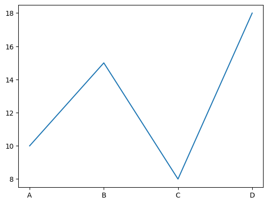
The easiest way of creating a Figure with only one Axes is by using the subplots method. This method returns the Figure and Axes object. Then we can call the method plot of the Axes object to plot data and the method show to display the figure on the screen.
fig, ax = plt.subplots() # Creates a Figure containing one Axes
ax.plot(['A','B','C','D'],[10,15,8,18]) # Plots data on the Axes
plt.show() # Show the figure
A Matplotlib Figure contains many elements which you may control to adjust your plot, see here. We will only see a few examples.
The Figure object keeps track of all the child Axes as well as of the auxillary elements such as titles, legends, colorbars and many more. The most frequenly used way of creating a Figure is, as we have seen before, through the subplots method.
fig, ax = plt.subplots() # Creates a Figure with one Axes
fig, axs = plt.subplots(2,2) # Creates a Figure with four Axes objects on a 2 x 2 grid.
fig, axs = plt.subplots(3,2) # Creates a Figure with six Axes objects on a 3 x 2 grid.
One can even gain a finer control of the position of the Axes objects as follows.
fig, axs = plt.subplot_mosaic([['left','right_top'],['left','right_bottom']])
This code creates a Figure with three Axes arranged in two columns. The left column contains only one Axes, the right column contains two stacked Axes.
When only one Axes is created, the subplots method returns the Figure and the individual Axes.
When multiple Axes are created, the subplots method returns the Figure and a list of the Axes created. Note, in fact, we use a variable ax in the first case and axs in the second case.
An Axes contains a region for plotting data and usually two (possibly three) Axis objects which represent the coordinate axes with ticks, lables and scales to represent the data in the Axes. We stress that an Axes is the container of the plotting region, while an Axis represents only the e.g., vertical and horizontal, axes in a plot.
It is probably easiest to directly see these element in concrete examples.
There are essentially two approaches to creating a plot with Matplotlib.
The object-oriented style, which consists of creating
FigureandAxesobjects as we have seen above, and calling their methods.The
pyplotstyle which relies onpyplotto implicitly create and manage theFigureandAxesobjects. Let us create the same plot using both styles.
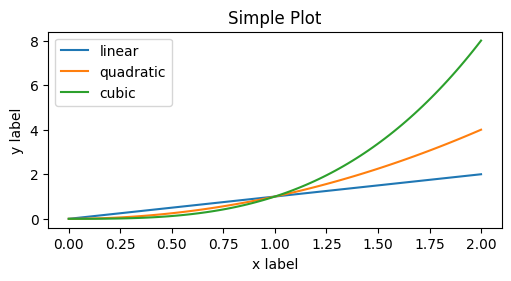
x = np.linspace(0, 2, 100) # Sample data.
# Here we create one Figure with one Axes
## You can also see examples of the arguments you can pass to the `subplots` method.
## For more information see here https://matplotlib.org/stable/api/_as_gen/matplotlib.pyplot.subplots.html#matplotlib.pyplot.subplots
fig, ax = plt.subplots(figsize=(5, 2.7), layout='constrained')
# On the Axes we plot three lines
ax.plot(x, x, label='linear') # a linear function
ax.plot(x, x**2, label='quadratic') # a quadratic function
ax.plot(x, x**3, label='cubic') # a cubic function
# Here is how we control the axis
ax.set_xlabel('x label') # Add an x-label to the Axes.
ax.set_ylabel('y label') # Add a y-label to the Axes.
ax.set_title("Simple Plot") # Add a title to the Axes.
ax.legend() # Add a legend.
<matplotlib.legend.Legend at 0x7fac0c56f880>
Now, let us do the same using the pyplot style.
x = np.linspace(0, 2, 100) # Sample data.
# We ask pyplot to create a Figure, but we will not interact directly with it.
plt.figure(figsize=(5, 2.7), layout='constrained')
# We interact with the Axes of the Figure only through pyplot
plt.plot(x, x, label='linear') # Plot some data on the (implicit) Axes.
plt.plot(x, x**2, label='quadratic') # etc.
plt.plot(x, x**3, label='cubic')
plt.xlabel('x label')
plt.ylabel('y label')
plt.title("Simple Plot")
plt.legend()
<matplotlib.legend.Legend at 0x7fac0c4a60a0>
We will use the object-oriented style, but the same things can be done using the pyplot style.
We will now see a number of examples of how to change the aesthetic of the plot, e.g., colors, line styles, subplots and so on.
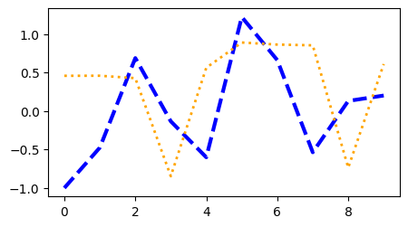
In the example below we manually set the color, linewidth and linestyle.
fig, ax = plt.subplots(figsize=(5, 2.7)) # Creates a Figure with one Axes
x = np.arange(10) # [0,9]
y1 = np.random.randn(10) # 10 random numbers
y2 = np.random.randn(10) # 10 random numbers
# We plot the cumulative sume of the 10 random numbers on the Axes.
# We pass arguments to the plot method to set line color, width and style.
l1 = ax.plot(x, np.cumsum(y1), color='blue', linewidth=3, linestyle='--')
l2 = ax.plot(x, np.cumsum(y2), color='orange', linewidth=2)
# The plot metod retuns a list of the lines it plots each time it is called.
# The lines in the list are objects of type Line2D (https://matplotlib.org/stable/api/_as_gen/matplotlib.lines.Line2D.html#matplotlib.lines.Line2D)
# By interacting with the line objects we can further adjust their characteristics.
l2[0].set_linestyle(':') # First (and only) line created in the second call of the plot method.
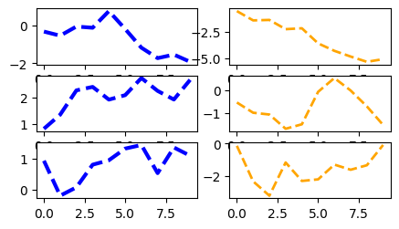
In the following example we put each line in its own sub-plot.
fig, axs = plt.subplots(3,2,figsize=(5, 2.7)) # Creates a Figure a 3x2 grid of Axes
# axs is now a 3 x 2 np.array, where each element is an Axes
x = np.arange(10) # [0,9]
y1 = np.random.randn(10) # 10 random numbers
y2 = np.random.randn(10) # 10 random numbers
y3 = np.random.randn(10) # 10 random numbers
y4 = np.random.randn(10) # 10 random numbers
y5 = np.random.randn(10) # 10 random numbers
y6 = np.random.randn(10) # 10 random numbers
# We plot the cumulative sume of the 10 random numbers on the Axes.
# We pass arguments to the plot method to set line color, width and style.
axs[0,0].plot(x, np.cumsum(y1), color='blue', linewidth=3, linestyle='--') # Row 0 column 0
axs[0,1].plot(x, np.cumsum(y2), color='orange',linewidth=2,linestyle='--') # Row 0 column 1
axs[1,0].plot(x, np.cumsum(y3), color='blue', linewidth=3, linestyle='--') # Row 1 column 0
axs[1,1].plot(x, np.cumsum(y4), color='orange',linewidth=2,linestyle='--') # Row 1 column 1
axs[2,0].plot(x, np.cumsum(y5), color='blue', linewidth=3, linestyle='--') # Row 2 column 0
axs[2,1].plot(x, np.cumsum(y6), color='orange',linewidth=2,linestyle='--') # Row 2 column 1
[<matplotlib.lines.Line2D at 0x7fac0bf898b0>]
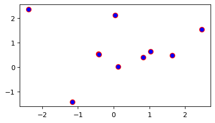
Here is a scatter plot.
fig, ax = plt.subplots(figsize=(5, 2.7))
d1, d2 = np.random.randn(2, 10) # Create two random arrays of 10 elements each
# Here is how to create a scatter plot. We give point size 50, and we ask the points to be blue with red border.
ax.scatter(d1, d2, s=50, facecolor='blue', edgecolor='red')
<matplotlib.collections.PathCollection at 0x7fac0c4ee790>
d1, d2, d3, d4 = np.random.randn(4, 10)
np.arange(10)
np.random.randn(10)
array([-0.7323409 , 3.48610777, 0.16284576, -1.1260133 , -0.33544956,
-0.510541 , -0.12775783, 0.15045047, 0.91144332, 1.28780625])
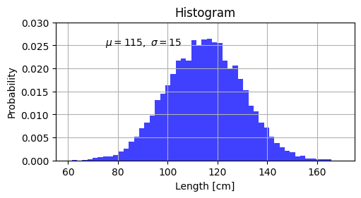
Here we add labels and text and we show another type of plot, the Histogram.
mu, sigma = 115, 15
x = mu + sigma * np.random.randn(10000) # Simulate normally distributed data
fig, ax = plt.subplots(figsize=(5, 2.7), layout='constrained')
# We create a histogram. We use 50 bins
ax.hist(x, 50, density=True, facecolor='blue', alpha=0.75)
ax.set_xlabel('Length [cm]') # Label of the x axis
ax.set_ylabel('Probability') # Label of the y axis
ax.set_title('Histogram') # Title of the plot
ax.text(75, .025, r'$\mu=115,\ \sigma=15$') # Annotates the plot with some text at point (75,0.25).
# The r preceeding the string indicates that the string should be understood as raw and not interpreted.
# This is done because we are passing LaTex code.
ax.axis([55, 175, 0, 0.03]) # Puts a grid on the axis.
ax.grid(True)
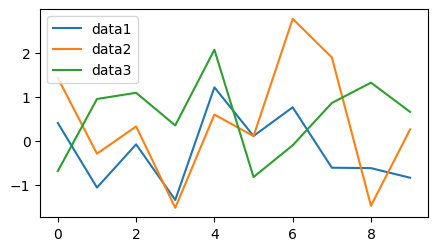
Here is how to add a legend.
fig, ax = plt.subplots(figsize=(5, 2.7))
d1, d2, d3 = np.random.randn(3, 10)
ax.plot(np.arange(len(d1)), d1, label='data1')
ax.plot(np.arange(len(d2)), d2, label='data2')
ax.plot(np.arange(len(d3)), d3, label='data3')
ax.legend(loc="upper left") # Put the legend in the upper left corner
<matplotlib.legend.Legend at 0x7fac0bd1dfd0>
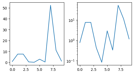
Here is how to use different scales.
# Two Axes on the same line (i.e., 1 x 2 grid of Axes)
fig, axs = plt.subplots(1, 2, figsize=(5, 2.7), layout='constrained')
y = 10**np.random.randn(10)
x = np.arange(10)
axs[0].plot(x, y) # We plot on the first Axis
# On the second Axis we plot using a log scale
axs[1].set_yscale('log')
axs[1].plot(x, y)
[<matplotlib.lines.Line2D at 0x7fac0bc25c70>]
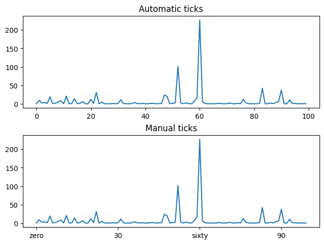
This is how to adjust the ticks of the axis.
fig, axs = plt.subplots(2, 1, layout='constrained')
x = np.arange(100)
y = 10**np.random.randn(100)
axs[0].plot(x, y)
axs[0].set_title('Automatic ticks')
axs[1].plot(x, y)
#axs[1].set_xticks(np.arange(0, 100, 30), ['zero', '30', 'sixty', '90'])
axs[1].set_xticks([0,30,60,90], ['zero', '30', 'sixty', '90']) # The first list contains the location of the ticks, the second list their labels.
axs[1].set_title('Manual ticks')
Text(0.5, 1.0, 'Manual ticks')
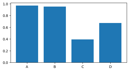
Here is an example of a bar plot with categorical data (see here for more examples).
fig, ax = plt.subplots(figsize=(5, 2.7), layout='constrained')
x = ['A', 'B', 'C', 'D']
y = np.random.rand(len(x))
ax.bar(x, y)
<BarContainer object of 4 artists>
Much more can be done with Matplotlib. Their introductory tutorial, on which this tutorial is based, provides some additional examples of Matplotlib features. Rather than getting an idea of every feature, it is probably best to learn some basic usage and then look for a specific solution in their documentation when the need arises.
1.12. Exercises#
Exercise 1.1
Given the following list of strings, create a dictionary where the keys are the strings that contain the letter “a” and the values are the lengths of those strings.
words = ["apple", "banana", "cherry", "date", "fig", "grape"]
Exercise 1.2
Given a list of numbers, create a dictionary where the keys are the odd numbers and the values are their squares.
nums = [0, 1, 2, 3, 4, 5, 6, 7, 8, 9]
Exercise 1.3
Given two lists of equal length, create a dictionary where the keys are elements from the first list and the values are elements from the second list.
Use, for instances:
keys = ["name", "age", "city"]
values = ["Alice", 25, "New York"]
Exercise 1.4
Given a string, for example text = "hello world" create a dictionary where the keys are characters and the values are the number of times each character appears in the string.
Exercise 1.5
Write a lambda function that adds two arguments, x and y.
Exercise 1.6
Write a function that takes as input the width and length of a rectangle and returns the area and the perimeter. Test if, for example, with a rectangle of with \(2\) and length \(4\).
Exercise 1.7
Write a function that takes as input the radius of a circle and returns the area and the perimeter. Test it, for example, with a radius of \(4\).
Exercise 1.8
Write a Python function to calculate the difference between the squared sum of the first \(n\) natural numbers and the sum of the squared first \(n\) natural numbers. That is \(\left(\sum_{i=1}^ni\right)^2-\sum_{i=1}^ni^2\). Test it, for example, with \(n=4\).
Exercise 1.9
Create a Python function which takes as first parameter a list of 2-d points in the Euclidean space and as second parameter an individual point in the Euclidean space. The list of points should be passed as a list of 2-d lists. The point should be a 2-d list. The function should return the list of Euclidean distances between the individual point and each point in the list.
Exercise 1.10
Write a function that computes the \(n\)-th Fibonacci number, given \(n\), and prints the output of every recursive call. Test it, for example, with \(n=5\).
Exercise 1.11
Write an iterative method for computing the \(n\)-th Fibonacci number. Test it, for example, with \(n=5\).
Exercise 1.12
Write a Python function to print all permutations of a given string. For example, when receiving the string “ABC” the function must return ['ABC', 'BAC', 'BCA', 'ACB', 'CAB', 'CBA'].
Exercise 1.13
The Tower of Hanoi problem consists of three poles or towers and \(N\) disks of different sizes. Each disk has a hole in the center so that the pole can slide through it. The original configuration of the disks is that they are stacked on one of the towers, in the order of decreasing size: the largest at the bottom, the smallest at the top. The goal of the problem is to move all the disks to a different pole while complying with the following three rules
Only one disk can be moved at a time
Only the disk at the top of a stack may be moved
A disk may not be placed on top of a smaller disk.
Write a python program that prints the instructions to solve the Tower of Hanoi problem for an arbitrary \(N\). Test it, for example, on the problem of moving \(N=3\) disks from tower \(1\) to tower \(2\) using tower \(3\) as intermediate tower.
Exercise 1.14
You are given a dictionary which stores information about rectangles.
This dictionary stores, for each rectangle, width and length as [width,length]. That is
rectangles = {"A":[2,5],"B":[4,3],"C":[10,7],"D":[5,8],"E":[9,12]}
Write some Python code that calculates the perimeter of each rectangle and write it to the file along with the width, length, and area.
Exercise 1.15
You are given a dictionary which stores information about rectangles.
This dictionary stores, for each rectangle, width and length as [width,length]. That is
rectangles = {"A":[2,5],"B":[4,3],"C":[10,7],"D":[5,8],"E":[9,12]}
Write some Python code that calculates the area of each rectangle and writes it to a file along with the width and length. In addition, at the end of the file, it reports the average width, length, and area.
Exercise 1.16
Using numpy.arange() generate a numpy.array containing the elements \([25,50,75, \ldots, 250]\).
Exercise 1.17
Using numpy.arange() generate a numpy.array containing the elements \([20,17,14, \ldots, 2,-1,-4]\).
Exercise 1.18
Using numpy.arange() generate a numpy.array containing the elements \([15.3, 16.2,\ldots, 20.7]\).
Exercise 1.19
Generate a numpy.array containing \(150\) number evenly spaced in the interval \([0.5,3.5]\).
Exercise 1.20
Consider the numpy.array generated by x = np.linspace(10,20,9). Create two arrays containing the first \(3\) and the reamining \(6\) elements of \(x\), respectively.
Exercise 1.21
Consider the numpy.arrays v1 = np.array([10,2,30,4]) and v2 = np.array([1,20,3,40]). Compute the products \(v_1^\top v_2\) and \(v_1v_2^\top\).